Hénon map
Introduction
The Hénon map is a two-dimensional, time-discrete, dynamical system given by the following equations:
We are dealing with a 2D, non linear map and we have two parameters a and b.
Let's start the study of this system, finding the more important characteristics such as fixed points, bifurcation diagrams, phase states and so on. Both analytic and numerical methods will be used, the plotting and numerical computation is done with matlab.

We will consider the parameters in the following range: \( a \in [0,1.5]\), b \(\in [-1,1]\).
Analysis of fixed point with varying parameters.
The fixed points of this system will be the couples \((x^*,y^*)\) such that:
where \(f(x,y)=y+1-ax^2\) and \(g(x,y)=bx\).
Fixed Points
Solving analitically:
We get a quadratic expression for \(x^*\):
from which we obtain the roots:
So, given \(a\neq0\), we have two fixed points \((x^*_\pm,y^*_\pm)\):
In order to be acceptable, the discriminant must be \(\gt0\), so we have that \((1-b)^2+4a>0\) from which follow \(a>-\frac{(1-b)^2}{4}\).
In our case, being \(b \in [-1,1]\) the quantity at the right of the disequation will be in the range \([-1,0]\), so \(a \in(0,1.5]\) will be always greater.
If \(a=0\), we find only one fixed point \((x^*,y^*)\) given by the following system:
from which we find the fixed point \((x^*,y^*)=(\frac{1}{1-b},\frac{b}{1-b})\) with \(b\ne1\).
To summarize, for the considered value of a and b, we have the following cases:
-
\(a=0\) and \(b=1\) no fixed points.
-
\(a=0\) e \(b\in[-1,1)\) : we find one fixed point:
\((x_1,y_1)=(\frac{1}{1-b},\frac{b}{1-b})\)
-
\(0<a\le1.5\) e \(b\in[-1,1]\) we find two fixed points:
\((x_1,y_1)=\frac{-(1-b)+\sqrt{(1-b)^2+4a}}{2a},\frac{-b(1-b)+b\sqrt{(1-b)^2+4a}}{2a}\)
\((x_2,y_2)=\frac{-(1-b)-\sqrt{(1-b)^2+4a}}{2a},\frac{-b(1-b)-b\sqrt{(1-b)^2+4a}}{2a}\)
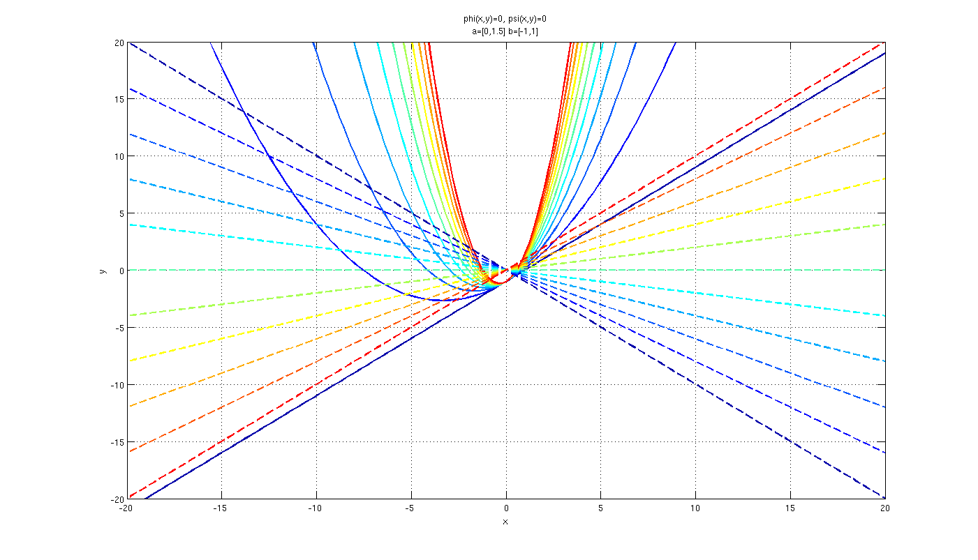
In order to give a geometrical visualization of the fixed points, it's convinient to define two function \(\phi(x,y)\) and \(\psi(x,y)\), whose zeros satisfy the condition neccesary to find the fixed point:
The fixed points will be the couples \((x,y)\) that cancel simultaneously the two functions \(\phi(x,y)\) and \(\psi(x,y)\). Because the zeros of these funtions defines curves on the plane \((x,y)\), the intersection of these curves will define the points where both are zero.
The values \((x,y)\) that cancel the function \(\psi(x,y)\) lay on the line crossing the origin with slope in the range \(b=[-1,1]\). The couples \((x,y)\) that cancel the function \(\phi(x,y)\) are on a parabula facing upward, the only exception is when \(a=0\), in this case the parabola collapse in a line.
This confirms what found earlier: we always have two interception between the parabola and the line, meaning we have two fixed point, unless in the case where \(a=0\). In this case we have only one intersection between two lines, except for when \(b=1\), where the two lines will be parallel so there are no interception
Stability of fixed points.
In order to study the stability of the fixed points \(\mathbf{x^*}\) we start by linearizing the differential equation near the fixed point, calculating the derivative of the function to obtain the behaviour around the point. Depending on the position of the eigenvalues with respect to the circumference of unit radius, we can determine the stability of the fixed point.
We proceed by calculating the Jacobian of the system:
To evaluate the stability we consider the eigenvalues of the Jacobian matrix:
The eigenvalues of the fixed point \((x^*,y^*)\) will be:
To evaluate the stability of the fixed point we have to check the position of the eigenvalues with respect to the circumference of unit radius.
Considering the case in which there is only one fixed point (when \(a=0\) and \(b\in[-1,1)\)) we get:
Being \(b\in[-1,1]\) the module of the eigenvalues will always be minor than \(1\), in particular for \(b\ge0\) the eigenvalues will be real and the module will be equal with opposite sign, so we get a stable flipping node.

For \(b<0\) the eigenvalues will be complex coniugate, so we get stable focus points as you can see in the picture below:

This happens except for \(b=-1\) where we can find a periodic behaviour with \(\omega=\frac{\theta}{2\pi}=\frac{\pi}{4\pi}=\frac{1}{4}\). Therfore we find a period 4 solution, as shown below:

Let's now consider the case where we have two fixed points: we approach the analysis using a numerical analysis. From the results we can conclude that, for the parameter's value considered, the second fixed point will always be a saddle node, while the first can have different type of stability, represented in the figure below.

Considering the parameter plane different type of stabulity are represented with different colors:
- Green: stable node.
- Blue: saddle node.
- Cyan: stable focus.
- Purple: non hyperbolic point.
Let's take a look on different trajectories corresponding to different equilibrium type:


Analysis of period two points
The period \(m\) orbit are determined by the following relation: \(x_{n+m} = x_n\). So, in order to find the period \(2\) point this relation must be true: \(x_{n+2}=x_n\), in other words we now consider the second iterate of the map:
In our case, having \(f(x,y)=y+1-ax^2\) and \(g(x,y)=bx\), the second iterate of the map will be:
Using the same reasoning as before, we proceed to find the fixed point of the second iterate, defining two functions \(\phi(x,y)\) and \(\psi(x,y)\):
The points \((x,y)\) that will cancel both functions will be fixed points of the 2nd iterate:
The zeros of the two functions will lay on two parabolas, one with a vertical axis and the other with a horizontal axis. The solutions of the system are the roots of the following polynomial:
from where we can obtain the \(y\) coordinates. The point of primary period two will be the fixed point of the second iterate that are not fixed point of the first iterate.
Let's look at an example, here we can see, marked in red, two fixed points regarding the first iterate, determined by the intersection from a parabola and a line, as explained before.

Let's now consider the second iterate: the fixed point will be determined by the intersection of two parabola, as said earlier. We can find the x coordinate of the fixed points as the zeros of the polynomial written above, which is drawn in blue in the picture, and than substitute in the system to find the y. In this case we find 4 points, but since we must discard those that are fixed point of the first iterate, we find 2 fixed point for the second iterate, marked in green.

In the following picture, are represented the value of the parameter \(a\) and \(b\) for which we can find limit cycle of period 2, coloured in red.

Stability of period 2 cycle
For the study of the period 2 cycle we use the chain rule:
In this case, since we are considering cycles of period 2 defined by the point \({\mathbf{x_0,x_1}}\), the two fixed points of primary period two, we can determine the stability of the cycle using the Jacobian of the map computed before:
To determine the stability we should calculate the aigenvalue of\(J^{(2)}\) and confider their position with respect to the unit circle:
Let's now visualize the module of the eigenvalues of the cycle of period two in the parameter plane: for each combination of parameter, the value of the module is represented by different colors. At the bottom of the image there is a bar showing the relation between the color and the value of the eigenvalue's module. Note that the color corresponding to \(-1\) means that there isn't cycle of period two for those parameters.
The module of the first eigenvalue \(\| \lambda_1 \|\) is plotted below.

The module of the second eigenvalue \(\| \lambda_2 \|\) is plotted below, note that in this case the value is always inside the unit cicle.

Finally, let's visualize the stability of the cycle of period 2 on the parameter plane. The meaning of the color is:
- Red: unstable.
- Green: stable, with real eigenvalues.
- Cyan: stable, with complex coniugate eigenvalues.
- Blue: there are no period 2 cycle.

Bifurcation diagrams
Keeping the parameter \(a\) fixed, with \(b \in [0.1,0.5]\):
- For \(a=0.5\)

- For \(a=1\)

- For \(a=1.5\)

Keeping the parameter \(b\) fixed, with \(a \in [0.5,1.5]\):
- For \(b=0.1\)

- For \(b=0.3\)

- For \(b=0.5\)

Phase state
Let's take a look at some phase state diagrams corresponding to different kinds of dynamics.
Period doubling
As seen in the bifurcation diagrams, there are some period doubling cascade, happening through flip bifurcations. Let's pick an example: we keep \(a\) fixed at \(0.5\), so we are looking at the first bifurcations diagram. Starting right before the bifurcation at \(b=0.183\) we have:
- Two fixed point for the first iterate:

- No fixed point on the second iterate:

- Therfore we have no period two solution, as we can see in the phase space:

Let's move just after the bifurcation happens, at \(b=0.184\). We find:
- Two fixed point for the first iterate:

- Two fixed point are born on the second iterate:

- In the phase state we now se a period two solution:

Those period doubling cascade are one of the route to chaos, as you can see on the bifurcation diagrams.
Plot a color diagram showing the divergence velocity of the points for \(a=0.2\) and \(b=1.01\)
For the parameter \(a=0.2\) and \(b=1.01\) we want to visualize on the phase state \(x_k\), \(y_k\) with \(x_k \in [-5,5]\) and \(y_k \in [-6,6]\) the velocity of divergence using different colours. To do that, for every point inside the plane, the number of iteration neccessary for the point to diverge is calculated. In this case for every point \((x,y)\) the number of iterations neccessary for the point to exit the circumference \(x^2+y^2>450\) has been stored, having a maximum number of \(450\) iteration before stopping. This is the result:

Trajectories
Now we draw some trajectories starting from \((x_0,y_0)=(0,0)\) for different parameters.
Trajectory for \((a,b)=(0.2,0.9991)\) with \((x_k,y_k) \in [-5,5]^2\)
=(0.2,0.9991).")
| 1° Iterate | $(x_1*,y_1*)$ $(x_2*,y_2*)$ |
$(2.2338,2.2318)$ $(-2.2383,-2.2363)$ |
$\lambda_1=1.5416 ~ \lambda_2=0.6481$ $ \lambda_1=1.5429 ~\lambda_2=-0.6476$ |
| 2° Iterate | $(x_1*,y_1*)$ $(x_2*,y_2*)$ |
$(2.2383,-2.2318)$ $(-2.2338,2.2363)$ |
$\lambda_1=0.5991 + 0.7995i ~\lambda_2=0.5991-0.7995i$ $\mid\lambda_i\mid=0.9991$ |
The fixed points of the first iterate are two saddle, the fixed points of the second iterate have complex coniugate eigenvalues whose module is approaching the stability boundary (Neimark-Saker bifurcation). Infact, increasing a little bit the value of \(b\):
=(2,−2).")
=(2,−2).")
Trajectory for \((a,b)=(0.2,-0.9999)\) with \(x_k \in [-0.2,1.2]\) and \(y_k \in [-1.2,0.2]\)
=(0.2,-0.9999).")
| 1° Iterate | $(x_1*,y_1*)$ $(x_2*,y_2*)$ |
$(0.4773,-0.4772)$ $(-10.4767,10.4757)$ |
$\lambda_1=-0.0954+0.9954i ~ \lambda_2=-0.0954-0.9954i$ $\lambda_1=3.9367~\lambda_2=0.2540$ |
| 2° Iterate | $(x_1*,y_1*)$ $(x_2*,y_2*)$ |
-- -- |
-- |
We find only two fixed points for the first iterate: one is a saddle and the other is a stable focus. It's the transition point between a stable focus and one non-hyperbolic point (for \(a=0.2,~b=-1\)). The eigenvalues are complex coniugate and at the boundary of stability (Neimark-Saker bifurcation). Let's see what happens if we increase \(b\) a little:


Trajectory for \((a,b)=(1.4,0.3)\) with \(x_k \in [-1.5,1.5]\) and \(y_k \in [-0.4,0.4]\)
=(1.4,0.3).")
| 1° Iterate | $(x_1*,y_1*)$ $(x_2*,y_2*)$ |
$(0.6313,0.1894)$ $(-1.1314,-0.3394)$ |
$\lambda_1=-1.9237 ~ \lambda_2= 0.1559$ $\lambda_1=3.2598 ~\lambda_2=-0.0920$ |
| 2° Iterate | $(x_1*,y_1*)$ $(x_2*,y_2*)$ |
$(0.9758,-0.1427)$ $(-0.4758,0.2927)$ |
$\lambda_1=-3.0101 ~\lambda_2=-0.0299$ |
For this parameters we get a strange attractor, that complex geometric figure in the picture. The behaviour is aperiodic and the trajectory is highly sensitive to initial conditions. Let's plot the series for the \(x\) coordinate with slightly different initial condition, for the blue series we start from \((1,1)\) and for the red from \((1.0001,1.0001)\):

As we can see after a small number of iteration, despite the initial conditions where almost the same, the two series are completely different.
Brute force bifurcation diagram

Different colors means different asyntotic behaviour. Dark blue (corresponding to 0 in the color scale) means divergence, red (10 in the color scale) means chaos or periodic solution with period grater than 9. Colors between 1 and 8 represent solution having the corresponding period.